Nyquist formula: relating data rate and bandwidth

This experiment looks at the relationship between data transmission rate, bandwidth, and modulation scheme, as described by the Nyquist formula.
It should take about 60-120 minutes to run this experiment, but you will need to have reserved that time in advance. This experiment uses wireless resources (either the sb3 or sb7 sandbox at ORBIT), and you can only use wireless resources on ORBIT/COSMOS during a reservation.
To reproduce this experiment on ORBIT/COSMOS, you will need an account, and you will need to have joined a project. You should have already uploaded your SSH keys to your profile. Finally, you must have reserved time on a sandbox at ORBIT (either sb3 or sb7), and you must run this experiment during your reserved time.
- Skip to Results
- Skip to Run my experiment
Background
The Nyquist formula gives the upper bound for the data rate of a transmission system by calculating the bit rate directly from the number of signal levels and the bandwidth of the system.
Specifically, in a noise-free channel, Nyquist tells us that we can transmit data at a rate of up to
$$ C = 2B\;log_2\;M$$
bits per second, where B is the bandwidth (in Hz) and M is the number of signal levels.
Nyquist is only an upper bound, and on the baseband signal bandwidth - the occupied transmission bandwidth for a wireless signal will further depend on how the signal is modulated onto a carrier frequency for wireless transmission. In this experiment, we will use PSK modulation, a digital modulation scheme in which the phase of a carrier signal is varied to represent different bits, or different groups of bits, and there are a discrete number of signal "levels" represented by different phase shifts.
In our experiment, the modulated wireless signal at RF will occupy a transmission bandwidth that is double the Nyquist bandwidth (at baseband):

The basic relationships implied by Nyquist will still hold:
- Doubling the data rate (C) and keeping the number of signal levels (M) the same, will double the bandwidth used (B), and
- Squaring the number of signal levels (M) and keeping the data rate (C) the same, will halve the bandwidth used (B).
In this experiment, we will send a constant amount of data over a wireless channel, with varying data rates (C) and number of signal levels (M). We will observe the effect of these variations on two metrics:
- The total time required to transfer the data, and
- The transmission bandwidth.
We expect to see that there are two ways to increase the speed of data transmission: using more bandwidth, or using more signal levels.
Results
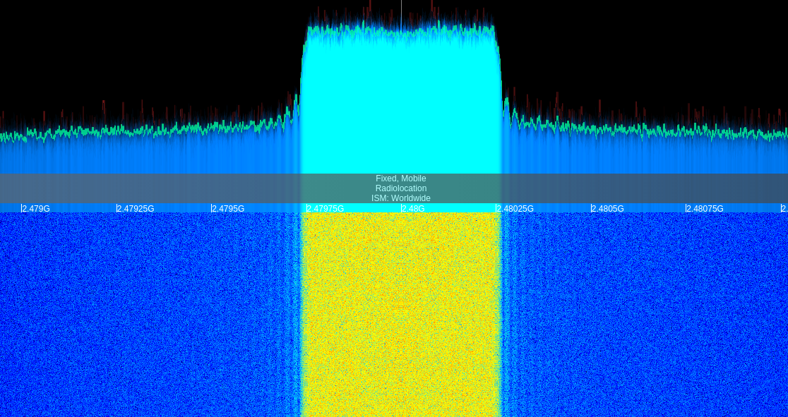
When we send 5 megabytes (40 Mbits) of data at a rate of 0.5 Mbps, using BPSK (2 signal levels), we see that about 0.5 MHz of bandwidth is used, and the total transmission takes a little over 80 seconds (the "ticks" on the display are 250 kHz apart):
However, if we change the bitrate to 2 Mbps, 2 MHz of bandwidth is used and the transmission takes about 20 seconds. To reduce the speed of data transfer by a factor of 4, we had to increase the bandwidth by a factor of 4:
Finally, on changing the constellation size to 4 points (squaring the number of signal levels relative to the first transmission), the transmission also takes about 20 seconds, but uses only 1 MHz, when transmitting at 2 Mbps:
Run my experiment
To run this experiment, you will need a reservation on either the sb3 or sb7 testbed on ORBIT. You will have to make your reservation in advance.
To reserve an ORBIT sandbox, visit http://orbit-lab.org. Click on "Log in", then log in. Then, click on "Control Panel". Use the calendar interface to request time on sb3 or sb7.
Set up testbed
At your reserved time, open a terminal and log in to the console of the testbed that you have reserved. For example, if you have reserved sandbox 3 on ORBIT,
ssh USERNAME@sb3.orbit-lab.org -i /PATH/TO/KEY
where USERNAME is your ORBIT/COSMOS username. Also specify the path to the key you have uploaded to ORBIT/COSMOS as the /PATH/TO/KEY.
If you are using sandbox 7 on ORBIT, log in to sb7.orbit-lab.org instead.
Then, you must load a disk image onto the testbed nodes. From the testbed console, run:
omf load -i gr-nyquist.ndz -t system:topo:all
This disk image has the GNU Radio software suite, and the ShinySDR spectrum analyzer, both of which we'll use for this experiment, pre-installed.
This process can take 5-10 minutes. Don't interrupt it in middle - you'll just have to start again, and it will only take longer.
If it's been successful, then once the process finishes running completely you should see output similar to:
 INFO exp:  -----------------------------
 INFO exp:  Imaging Process Done
 INFO exp:  2 nodes successfully imaged - Topology saved in '/tmp/omf-pxe_slice-2014-02-04t16.38.52-05.00-topo-success.rb'
 INFO exp:  -----------------------------
Sometimes, transient errors can cause the process to fail - if you haven't successfully imaged 2 nodes, wait a few minutes and try again.
Then, turn on your nodes with the following command:
omf tell -a on -t system:topo:all
Wait a few minutes for your testbed nodes to turn on, then continue with the experiment.
Prepare your receiver
Open a new terminal window, and run the following command to tunnel the ShinySDR ports between your laptop and the receiver node. For example, if using "sb3":
ssh -L 8100:node1-2:8100 -L 8101:node1-2:8101 USERNAME@sb3.orbit-lab.org -i /PATH/TO/KEY
again, using the correct USERNAME, /PATH/TO/KEY, and substituting sb3.orbit-lab.org for the hostname of the console of the testbed that you have reserved.
Then, in that terminal window (which should now be logged in to your testbed console), log on to the receiver node:
ssh root@node1-2
On the receiver node, run
cd ~/shinysdr

# Run shiny server
python -m shinysdr.main ~/.shiny
This last command should start the Shiny server, which, when it is running successfully, will say something like:
INFO:shinysdr:ShinySDR is ready.
INFO:shinysdr:Visit http://localhost:8100/ShinySDR/
In a Google Chrome incognito browser window (should be a recent version of Chrome), open the URL that is shown in the Shiny server output. (http://localhost:8100/ShinySDR/).
Configure your Shiny window as follows (you may find it useful to right-click and slow down this video, and pause often so you can follow along):
- Click on the "hamburger" icon in the top left corner to open the menu, if it isn't already open.
- Un-select the "Frequency DB" display to hide that display if it is showing.
- Select the "Radio Config" display if it isn't showing.
- In the "Radio Config" section, set the "RF Source" to "OsmoSDR", the "Antenna" to "TX/RX", and the "Center Frequency" to 2,480,000,000 (2.48 GHz).
- Note the "Gain" slider in the "Radio Config" section. You may have to increase the gain later if you aren't able to see the transmission in the ShinySDR window.
- Check the "Use DC Cancellation" box, but don't worry if it doesn't stay checked. This setting is not strictly required.
- Use the "Options" section to adjust the dynamic range and reference level of the visualization so that you can see the noise floor and there is about 60-80 dB of range.
- Click on the "hamburger" again to close the menu.
Prepare your transmitter
In a second terminal window, log in to the node that will act as transmitter. First, log in to the testbed console:
ssh USERNAME@sb3.orbit-lab.org -i /PATH/TO/KEY
again, using the correct USERNAME, /PATH/TO/KEY, and substituting sb3.orbit-lab.org for the hostname of the console of the testbed that you have reserved.
Then, from there, log in to the transmitter node:
ssh root@node1-1
To generate a PSK signal, we will run the following command in the transmitter terminal window:
time /usr/local/share/gnuradio/examples/digital/narrowband/benchmark_tx.py -f 2480e6 -r 0.5e6 -M 5 -p 2 --excess-bw=0.05
where
-fis used to set the frequency at which to transmit,-rspecifies the bitrate at which to transmit, in bits per second,-Mspecifies the total amount of data to transmit, in megabytes,-pindicates how many constellation points (signal levels) to use (must be a power of 2),--excess-bwis a filter setting that determines how much "extra" leakage bandwidth the signal is allowed to use.
Later in this experiment, we will modify the values of the -r and -p arguments.
(If you aren't able to see any transmission in the ShinySDR window, see the Notes section for advice on increasing the gain.)
When we run this, we see that about 0.5 MHz of bandwidth is used (the "ticks" on the display are 250 kHz apart), and the total transmission takes a little over 80 seconds (look at the "real" time in the final output on the transmitter):
However, if we change the bitrate to 2 Mbps, 2 MHz of bandwidth is used and the transmission takes about 20 seconds:
time /usr/local/share/gnuradio/examples/digital/narrowband/benchmark_tx.py -f 2480e6 -r 2e6 -M 5 -p 2 --excess-bw=0.05
Finally, changing the constellation size to 4 points, the transmission still takes about 20 seconds, but uses only half the bandwidth, 1 MHz, when transmitting at 2 Mbps:
time /usr/local/share/gnuradio/examples/digital/narrowband/benchmark_tx.py -f 2480e6 -r 2e6 -M 5 -p 4 --excess-bw=0.05
Notes
If you aren't able to see the transmission in the ShinySDR window, you may have to make some adjustments; some testbeds may have more attenuation (signal loss) between the transmitter and receiver, and so the default gain settings are not sufficient to see the transmission. You can increase the gain on both the receiver and the transmitter:
- To increase the gain on the receiver, use the gain slider in the "Radio Config" window in ShinySDR.
- To increase the transmission amplitude on the transmitter, run the transmitter with
--tx-amplitude=0.8at the end of the command, each time you run it. For example:
time /usr/local/share/gnuradio/examples/digital/narrowband/benchmark_tx.py -f 2480e6 -r 0.5e6 -M 5 -p 2 --excess-bw=0.05 --tx-amplitude=0.8
Exercise
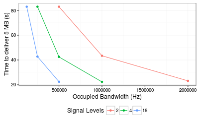
Using the same procedure as described above, measure the time to deliver 5 MB and the occupied transmission bandwidth for each of the following experiments (i.e. fill in the table):
| Number of signal levels | Bitrate (bps) | Time to deliver 5MB (s) | Occupied bandwidth (Hz) |
| 2 | 500,000.00 | ||
| 2 | 1,000,000.00 | ||
| 2 | 2,000,000.00 | ||
| 4 | 500,000.00 | ||
| 4 | 2,000,000.00 | ||
| 4 | 1,000,000.00 | ||
| 16 | 500,000.00 | ||
| 16 | 2,000,000.00 | ||
| 16 | 1,000,000.00 |
Create a scatter plot of your experiment data. Put time to deliver 5MB on the y-axis, occupied bandwidth on the x-axis, and have the color of each data point indicate the number of signal levels. Add lines connecting data points of the same color. For example: