UAV-assisted wireless localization

You've been asked to contribute your machine learning expertise to a crucial and potentially life-saving mission.

A pair of hikers has gone missing in a national park, and they are believed to be critically injured. Fortunately, they have activated a wireless locator beacon, and it transmits a constant wireless signal from their location. Unfortunately, their beacon was not able to get a satellite fix, so their GPS position is not known.

To rescue the injured hikers, therefore, their location must be estimated using the signal strength of the wireless signal from the beacon: when a radio receiver is close to the beacon, the signal strength will be high. When a radio receiver is far from the beacon, the signal strength will be lower. (The relationship is noisy, however; the wireless signal also fluctuates over time, even with a constant distance.)

You are going to fly an unmanned aerial vehicle (UAV) with a radio receiver around the area where they were last seen, and use the received wireless signal strength to fit a machine learning model that will estimate the hikers' position. Then, you'll relay this information to rescuers, who will try to reach that position by land. (Unfortunately, due to dense tree cover, the UAV will not be able to visually confirm their position.)

There is a complication, though - the UAV has a limited battery life, and therefore, limited flight time. You'll have to get an accurate estimate of the hikers' position in a very short time!

To run this experiment, you should already have an account on AERPAW with the experimenter role, be part of a project, have all the necessary software to work with AERPAW experiments. See: Hello, AERPAW.

Background

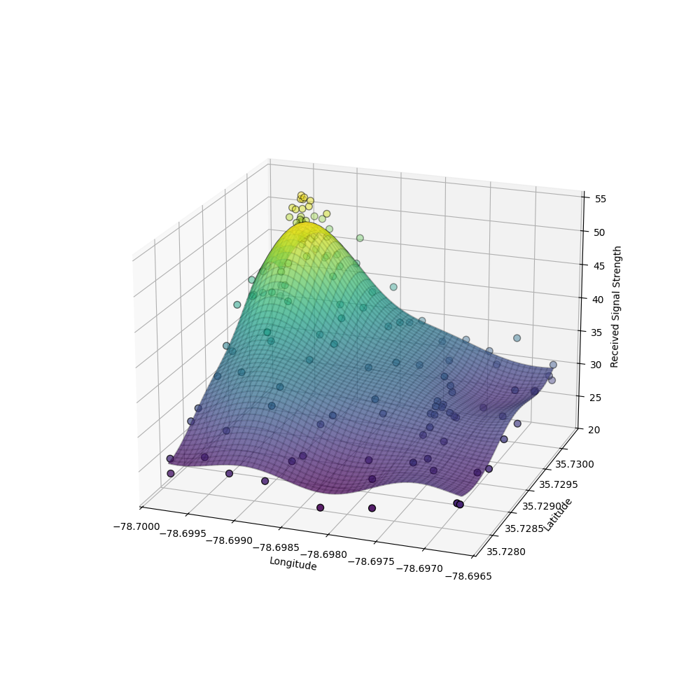
We are going to estimate the hikers' position based on the premise that the received signal strength is highest when the UAV is at the same latitude and longitude as the hikers.

We will frame our machine learning problem as follows:

• features X: latitude, longitude
• target variable y: received signal strength

In other words, given a coordinate (latitude and longitude) we want to predict the received signal strength at that location.

You can learn more about the problem, and our approach to solving it with a Gaussian Processing Regression, using the following Colab notebook:

However, we don't care as much if our model is bad at predicting the signal strength in places where it is low! Our true goal is to predict where the target variable will be highest. We will decide how "good" our model is by computing the mean squared error of the position estimate: the distance between the true location of the hikers, and the coordinate that our model predicts has the highest received signal strength.

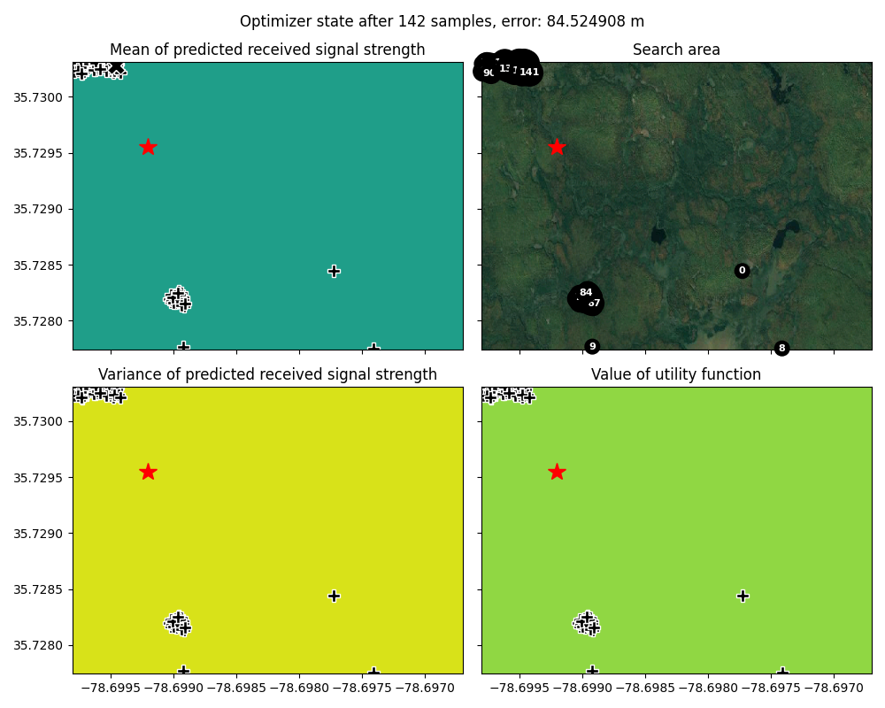
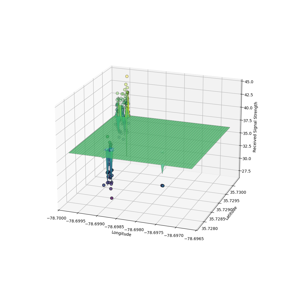
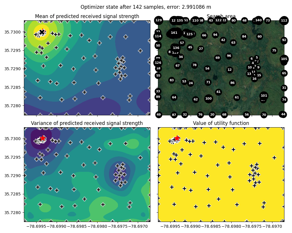
There are some "pathological" behaviors we will want to avoid. A combination of

• over-emphasis on "exploiting" areas of the search space where we have observed the highest signal strength so far,
• and mis-attributing the noise in the received signal strength as signal variation due to distance, causing the optimizer to choose a too-narrow kernel in order to fit this noise

can make our model get "stuck" in an area far from the true maximum, like this:

We could adjust the kappa hyperparameter of the Bayesian optimization to influence the search behavior. But, then we may spend too much time "exploring" the search space, instead of focusing on the area where the signal strength is highest:

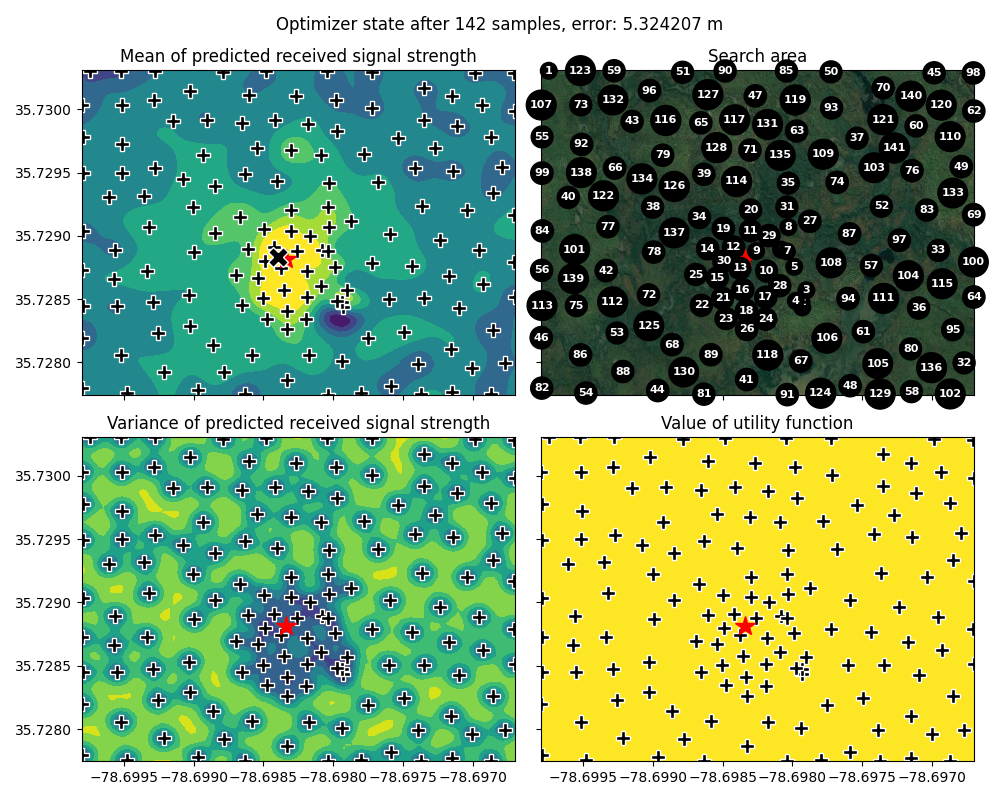
If the search time is large relative to the search area, we'll get reasonably close to the "true" position anyway. But if we don't have much time, or have a large area to search, this will be very inefficient.

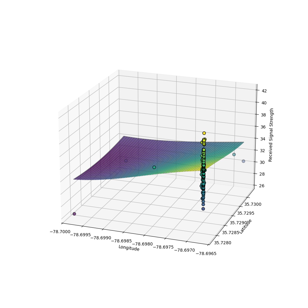
We can address the problem of mis-attributing noise as signal variation due to distance by adding a White Kernel to our Gaussian Process Regression, telling it to explicitly model the effect of noise in its estimate.

However, if it estimates a noise level that is too high, then we will have the opposite problem - it will mis-attribute signal variation that is due to distance, as random noise:

We are looking for the settings that will learn a function that is "just right" - not too smooth, not too noisy - regardless of the location of the transmitter, and that will learn this function quickly!

Run my experiment

Start an experiment

In this experiment, you are going to set up an experiment with two mobile vehicles: one aerial vehicle (UAV) and one ground vehicle (UGV).

Note: If you are working as a group, one member of the group should complete the steps in "Add members and resources to your experiment" on behalf of the entire group, to create a single AERPAW experiment to be used by all members of the group. Then, each group member can (separately) run the experiment from "Access experiment resources" until the end.

Add members and resources to your experiment

First, log in to the AERPAW Experiment Portal. Click on "Projects" in the navigation bar, and find the project that you are a member of; click on it to open the project overview. Click on the "Create" button in the "Experiments" section.

Now, you will have to fill in some details about your experiment:

• Select "Canonical" as the experiment type. This setting is required.
• Give your experiment a short title: you may use the template hello_username, e.g. hello_ffund in my case, for the experiment name
• Enter your university name for "host institution"
• For "title of your sponsored project", write "NA", and specify that there is no grant number
• For "Name of the lead experimenter", specify the name of your instructor or research advisor who is supervising your use of AERPAW. And, put their email address in the "email of the lead experimenter" field
• in the "Keywords: section, you can use: wireless, uav, aerpaw
• For "ultimate end destination" select "Development only".
• You can select "No" for urgency and "No" for sharing data.
• and in "expected behavior of the vehicles" you can write: "Hello AERPAW"

Then, click "Create canonical experiment".

Note: If you have omitted any field in the form, then an error is raised when you "Create canonical experiment". However, the experiment is still created and you can return to the project page, find your experiment by name, click on it, and proceed to the next step.

From the experiment page, you will add members and resources to the experiment:

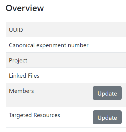
Click on the "Update" button next to "Members".

1. Select your course instructor or research advisor, click on the arrow to the move them to the list of "Chosen Members".
2. If you have team members or peers you are working with, click on the arrow to move them to the list of "Chosen Members".

Then click "Save". (Your advisor and team members will only have access to your experiment resources if you added them to the experiment at this stage - before deploying the resources.)

Back on the experiment page, click on the "Update" button next to "Targeted Resources". Then, click "Add/Update".

On this page, you will add two resources to the experiment:

• under "Portable Resources", toggle LPN1
• and then LPN2

Make sure that LPN1 has node number 1, and LPN2 has node number 2.

Click "Save". Then, you will modify each of the nodes by clicking "Modify" -

• for node number 1 (this will be the UAV, which is assumed to be the first vehicle in the rest of the instructions), change the name to "UAV", change the "Node Vehicle" property to "vehicle_uav" and click "Save"
• for node number 2 (this will be the UGV, which is assumed to be the second vehicle in the rest of the instructions), change the name to "UGV", change the "Node Vehicle" property to "vehicle_ugv" and click "Save"

Click "Back to Experiment", then "Initiate Development".

You will receive an email with the subject "Request to initiate development session". You must then wait until you receive another email notification indicating that the development session is active.

Access experiment resources

Once you receive notification that your development session is active, when you return to your experiment page in the Experiment Web Portal, you will see a "Linked files" section with two files - click the "download" link next to each to download these files to your computer.

At this stage, you are ready to access experiment resources! To access resources on AERPAW, you need to establish a connection to them in three steps:

• Start a VPN - none of the later steps will work unless your VPN connection to AERPAW is established successfully.
• Start an SSH session to the AERPAW experiment console, with port forwarding, and connect QGroundControl to this SSH session
• Start one or more SSH sessions to the AERPAW resources

Start VPN

To start the VPN connection, you will need the file with .ovpn extension that you downloaded from the experiment portal page. Then, your next steps will depend on your OS.

On Linux - start VPN

Suppose your .ovpn file is named aerpaw-XM-X0000-common.ovpn. On Linux, you would run

sudo openvpn aerpaw-XM-X0000-common.ovpn

in a terminal (from the same directory where you have downloaded the file). If it is successful, you should see

2024-07-12 13:08:04 TUN/TAP device tap0 opened
2024-07-12 13:08:04 Initialization Sequence Completed

in the output. Leave this running, and in a second terminal window, run

sudo dhclient tap0

or

sudo dhcpcd -b tap0

(depending on which DHCP client is installed on your system). Use

ip addr

to make sure that tap0 is assigned an IPv4 address.

On Mac - start VPN

For Mac OS, the recommended VPN software is Tunnelblick. With Tunnelblick running, open the Finder. Drag and drop the .ovpn file onto the Tunnelblick icon in the menu bar. You may be asked if the configuration should be shared or private (either is fine!) and you may have to give administrator authorization to install the configuration.

Once the VPN configuration is installed in Tunnelblick, when you click on the Tunnelblick icon in the menu bar, you should see a "Connect" option for this configuration. You can click on this "Connect" option to start the VPN connection. Wait several seconds after the connection is established and it turns "green" before you proceed to the next step, since it takes some additional time to assign an address to the VPN interface.

Note: For Mac users: AERPAW VPNs use something called a tap interface. On some versions of MacOS you may need to take some additional steps in order to use a tap interface - refer to the instructions here for your specific OS version.

On Windows - start VPN

When you run OpenVPN, an icon should appear in the system tray. From OpenVPN, use "Import > Import file" to import the .ovpn file, then click "Connect".

Start SSH Port Forwarding + Connect QGroundControl

When the VPN is running, you can connect QGroundControl to your AERPAW experiment! For this, you will need the Manifest.txt file you downloaded. Open it and find the address of the "OEO Console". (This will follow the pattern 192.168.X.62 where the value of X is different for each AERPAW experiment - so you need to check the manifest to find out the value in your experiment.)

Then, assuming you had generated an AERPAW key at ~/.ssh/id_rsa_aerpaw following the instructions above, open your terminal and run

ssh -i ~/.ssh/id_rsa_aerpaw -L 5760:127.0.0.1:5760 root@192.168.X.62

where in place of the address with the X, you use the address you identified earlier in the manifest. You may be prompted for the passphrase for your key, if you set a passphrase when generating the key.

The first time you log in to a new host, your computer may display a warning similar to the following:

The authenticity of host can't be established.
RSA key fingerprint is SHA256:FUNco2udT/ur2rNb2NnZnUc8s2v6xvNdOFhFFxcWGYA.
Are you sure you want to continue connecting (yes/no)?

and you will have to type the word yes and hit Enter to continue.

When this is successful, you should see that the terminal prompt indicates that you are logged in to the experiment console, like this:

root@OEO-CONSOLE:~$ 

Run

cd; ./startOEOConsole.sh

This will display a table showing all of the vehicles in your experiment, and their current state. You should see two vehicles, with ID 1 and ID 2, like this:

| ID | armed | mode      | alt    | heartbeat | gps | screens |
|----|-------|----------|--------|-----------|-----|---------|
| 1  | 0     | ALT_HOLD | -0.017 | 1987      | 6   | []      |
| 2  | 0     | MANUAL   | -0.166 | 1868      | 6   | []      |

Leave this running - later, you will need to run some additional commands in this window.

Now you can connect QGroundControl to your experiment. In QGroundControl,

• Open the QGroundControl application menu (Q in the upper left corner)
• Click "Application Settings > Comm Links > Add"
• Fill in the fields as follows:
  • Name: Remote Link
  • Type: TCP
  • Server Address: 127.0.0.1
  • Port: 5760
• Check "Automatically Connect On Start".

Click OK, then click on the link to highlight it (it will turn bright yellow), then click "Connect" on the bottom. Then, click the "Back" button to return to the main application.

Now, when you open QGroundControl, you should see the two vehicles in your experiment, in their start position (at the Lake Wheeler Road Field Laboratories at North Carolina State University).

Set up experiment on UAV and UGV VMs

Now, we will configure applications that will run in the experiment - the radio transmitter (on UGV) and radio receiver (on UAV), and the Bayes search on the UAV.

Inside the SSH session on the UAV (node 1 in the experiment), install the bayesian-optimization package, which we will use to implement a Bayes search:

# run on E-VM-M1 (UAV node)
python3 -m pip install --target=/root/Profiles/vehicle_control/RoverSearch bayesian-optimization==2.0.0 numpy==1.26.4 scikit_learn==1.5.2

Download the rover-search.py script:

# run on E-VM-M1 (UAV node)
wget https://raw.githubusercontent.com/teaching-on-testbeds/uav-wireless-localization/refs/heads/main/rover_search.py -O  /root/Profiles/vehicle_control/RoverSearch/rover_search.py

and the signal power plotting script:

# run on E-VM-M1 (UAV node)
wget https://raw.githubusercontent.com/teaching-on-testbeds/hello-aerpaw/refs/heads/main/resources/plot_signal_power.py -O  /root/plot_signal_power.py

Still in the SSH session on the UAV (node 1 in the experiment), set up the applications that will run during our experiment - a radio receiver and a vehicle control script that implements our search with Gaussian Process Regression and Bayesian Optimization:

# run on E-VM-M1 (UAV node)
cd /root/Profiles/ProfileScripts/Radio 
cp Samples/startGNURadio-ChannelSounder-RX.sh startRadio.sh 

cd /root/Profiles/ProfileScripts/Vehicle
cp Samples/startRoverSearch.sh startVehicle.sh

cd /root

We will also change one parameter of the radio receiver. Run:

# run on E-VM-M1 (UAV node)
sed -i 's/^SPS=.*/SPS=8/' "/root/Profiles/ProfileScripts/Radio/Helpers/startchannelsounderRXGRC.sh"

Then, open the experiment script for editing

# run on E-VM-M1 (UAV node)
cd /root
nano /root/startexperiment.sh

and at the bottom of this file, remove the # comment sign (if there is one) next to ./Radio/startRadio.sh and ./Vehicle/startVehicle.sh, so that the end of the file looks like this:

./Radio/startRadio.sh
#./Traffic/startTraffic.sh
./Vehicle/startVehicle.sh

Hit Ctrl+O and then hit Enter to save the file. Then use Ctrl+X to exit and return to the terminal.

Now we will set up the UGV.

Inside an SSH session on the UGV (node 2 in the experiment), set up the applications that will run during our experiment - a radio transmitter and a vehicle GPS position logger:

# run on E-VM-M2 (UGV node)
cd /root/Profiles/ProfileScripts/Radio 
cp Samples/startGNURadio-ChannelSounder-TX.sh startRadio.sh 

cd /root/Profiles/ProfileScripts/Vehicle
cp Samples/startGPSLogger.sh startVehicle.sh

cd /root

We will also change one parameter of the radio transmitter. Run:

# run on E-VM-M2 (UGV node)
sed -i 's/^SPS=.*/SPS=8/' "/root/Profiles/ProfileScripts/Radio/Helpers/startchannelsounderTXGRC.sh"

Then, open the experiment script for editing

# run on E-VM-M2 (UGV node)
cd /root
nano /root/startexperiment.sh

and at the bottom of this file, remove the # comment sign (if there is one) next to ./Radio/startRadio.sh and ./Vehicle/startVehicle.sh, so that the end of the file looks like this:

./Radio/startRadio.sh
#./Traffic/startTraffic.sh
./Vehicle/startVehicle.sh

Hit Ctrl+O and then hit Enter to save the file. Then use Ctrl+X to exit and return to the terminal.

Set up steps in experiment console

Note: a video of this section is included at the end of the section.

On the experiment console, run

# run on OEO-CONSOLE VM
./startOEOConsole.sh

and add a column showing the position of each vehicle; in the experiment
console run

# run on OEO-CONSOLE VM, inside the experiment console process
add vehicle/position

and you will see a vehicle/position column added to the end of the table.

Then, in this experiment console window, set the start position of the
UGV (node 2):

# run on OEO-CONSOLE VM, inside the experiment console process
2 start_location 35.729 -78.699

and restart the controller on the UGV, so that the change of start location will take effect:

# run on OEO-CONSOLE VM, inside the experiment console process
2 restart_cvm

If you are also watching in QGroundControl: In QGroundControl, the connection to the UGV may be briefly lost. Then it will return, and the UGV will be at the desired start location.

Even if you are not watching in QGroundControl, you will see in the vehicle/position column in the experiment console that the UGV (node 2) is at the position we have set.

Rover search experiment with default position and default model

Now we are ready to run an experiment!

Reset

Note: a video of this section is included at the end of the section.

Start from a "clean slate" - on the UAV VM (node 1) and the UGV VM (node
2), run

# run on E-VM-M1 (UAV node) and ALSO on E-VM-M2 (UGV node)
cd /root
./stopexperiment.sh

to stop any sessions that may be lingering from previous experiments.

You should also reset the virtual channel emulator in between runs - on
either VM (node 1 or node 2) run

# run on E-VM-M1 (UAV node) OR on E-VM-M2 (UGV node)
./reset.sh

Start experiment

Note: a video of this section is included at the end of the section.

On the UGV VM (node 2), run

# run on E-VM-M2 (UGV node)
cd /root
./startexperiment.sh

In the terminal in which you are connected to the experiment console
(with a table showing the state of the two vehicles) run

# run on OEO-CONSOLE VM, inside the experiment console process
2 arm

In this table, for vehicle 2, you should see a "vehicle" and "txGRC"
entry in the "screens" column.

On the UAV VM (node 1), run

# run on E-VM-M1 (UAV node)
cd /root
./startexperiment.sh

and wait a few moments, until you see the new processes appear in the
"screens" column of the experiment console.

Then check the log of the vehicle navigation process by running (on the
UAV VM, node 1):

# run on E-VM-M1 (UAV node)
tail -f Results/$(ls -tr Results/ | grep vehicle_log | tail -n 1 )

You should see a message

Guided command attempted. Waiting for safety pilot to arm

When you see this message, you can use Ctrl+C to stop watching the
vehicle log.

In the experiment console, run

# run on OEO-CONSOLE VM, inside the experiment console process
1 arm

to arm this vehicle. It will take off, reach altitude 50, and begin to
search for the UGV.

You can monitor the position of the UAV by watching the flight in
QGroundControl, or you can watch the position in the experiment console.

While the search is ongoing, monitor the received signal power by
running (on the UAV VM, node 1):

# run on E-VM-M1 (UAV node)
python3 plot_signal_power.py

and confirm that you see a stream of radio measurements, and that the
signal is stronger when the UAV is close to the UGV.

The experiment will run for 5 minutes from the time that the UAV reaches
altitude. Then, the UAV will return to its original position and land.

When you see that the "screens" column in the experiment console no longer includes a "vehicle" entry for the UAV (node 1), its "mode" is LAND, and its altitude is very close to zero, then you know that the experiment is complete. You must wait for the experiment to completely finish, because the data files are only written at the end of the experiment.

Transfer data from AERPAW for analysis

Once your experiment is complete, you can transfer a CSV file of the search progress and the final optimizer state from AERPAW to your own laptop, for further analysis.

On the UAV VM (node 1), run

# run on E-VM-M1 (UAV node)
echo /root/Results/$(ls -tr Results/ | grep ROVER_SEARCH | tail -n 1 )

to get the name of the CSV file.

On the UAV VM (node 1), run

# run on E-VM-M1 (UAV node)
echo /root/Results/$(ls -tr Results/ | grep opt_final | tail -n 1 )

to get the name of the "pickled" optimizer file.

Then, in a local terminal (not inside any SSH session), cd to a directory where you have write access (if necessary) and run

# run on your local terminal -NOT inside an SSH session
scp -i ~/.ssh/id_rsa_aerpaw root@192.168.X.1:/root/Results/ROVER_SEARCH_DATA_XXXXXX.csv ROVER_SEARCH_DATA_default.csv

where

• in place of the address with the X, you use the address you
  identified in the manifest,
• in place of the file name with the XXXXXX in the filename,
  you substitute the rover search CSV filename you identified above

Also run

# run on your local terminal -NOT inside an SSH session
scp -i ~/.ssh/id_rsa_aerpaw root@192.168.X.1:/root/Results/opt_final_XXXXXX.pickle opt_final_default.pickle

where

• in place of the address with the X, you use the address you
  identified in the manifest,
• in place of the file name with the XXXXXX in the filename,
  you substitute the "pickled" optimizer filename you identified above

You may be prompted for the passphrase for your key, if you set a
passphrase when generating the key.

After you run these scp commands, you should have a ROVER_SEARCH_DATA_default.csv file and an
opt_final_default.pickle file on your laptop.

Analyze experiment results

To analyze the experiment results, open the following Colab notebook:

Execute the first few cells in that notebook, to import libraries and functions.

Then, use the file browser in Google Colab to upload the ROVER_SEARCH_DATA_default.csv file and opt_final_default.pickle file to Colab.

Run the "Analyze experiment results from "default" experiment" section to visualize the search.

Rover search with new location and default model

Next, you will re-run the experiment, but with the rover at a different location. Use the cell at the beginning of the "Analyze results from rover search with new location" section of the Colab notebook to generate a "personal" new start position for the rover.

Now, you will re-do the "Rover search experiment" section. You will:

• Repeat "Set up steps in experiment console", but use the "personal" latitude and longitude generated in the Colab notebook for your net ID.
• Repeat the "Run experiment" steps (including "Reset" and "Start experiment").

Once your experiment is complete, you will transfer the CSV file of the search progress and the final optimizer state from AERPAW to your own laptop, for further analysis.

On the UAV VM (node 1), run

# run on E-VM-M1 (UAV node)
echo /root/Results/$(ls -tr Results/ | grep ROVER_SEARCH | tail -n 1 )

to get the name of the new CSV file.

On the UAV VM (node 1), run

# run on E-VM-M1 (UAV node)
echo /root/Results/$(ls -tr Results/ | grep opt_final | tail -n 1 )

to get the name of the new "pickled" optimizer file.

Then, in a local terminal (not inside any SSH session), cd to a directory where you have write access (if necessary) and run

# run on your local terminal -NOT inside an SSH session
scp -i ~/.ssh/id_rsa_aerpaw root@192.168.X.1:/root/Results/ROVER_SEARCH_DATA_XXXXXX.csv ROVER_SEARCH_DATA_new.csv

where

• in place of the address with the X, you use the address you
  identified in the manifest,
• in place of the file name with the XXXXXX in the filename,
  you substitute the rover search CSV filename you identified above

Also run

# run on your local terminal -NOT inside an SSH session
scp -i ~/.ssh/id_rsa_aerpaw root@192.168.X.1:/root/Results/opt_final_XXXXXX.pickle opt_final_new.pickle

where

• in place of the address with the X, you use the address you
  identified in the manifest,
• in place of the file name with the XXXXXX in the filename,
  you substitute the "pickled" optimizer filename you identified above

You may be prompted for the passphrase for your key, if you set a
passphrase when generating the key.

After you run these scp commands, you should have a ROVER_SEARCH_DATA_new.csv file and an
opt_final_new.pickle file on your laptop. These are the results for the default model, but
with the rover at the new location.

Upload these files to the Colab notebook.

Then, in the rest of the "Analyze results from rover search with new location" section you will repeat the analysis for your new experiment (with the "hikers' position" at this new location).

Rover search with new location AND customized model

Finally, you will re-run the experiment, but you may modify the kernel function and/or the utility function of the Bayesian optimization, in order to satisfy the specific requirements:

• Try to achieve 10m or less estimation error by
  the end of the five-minute flight.
• and, your fitted model should not show signs of severe overfitting
  or under-modeling - it should show a reasonable approximation of the
  function of signal strength vs position over the search space.

Currently, the optimizer is configured as:

    utility = acquisition.UpperConfidenceBound()

    optimizer = BayesianOptimization(
      f=None,
      pbounds={'lat': (MIN_LAT, MAX_LAT), 'lon': (MIN_LON, MAX_LON)},
      verbose=0,
      random_state=0,
      allow_duplicate_points=True,
      acquisition_function = utility
    )
    # set the kernel
    kernel = RBF()
    optimizer._gp.set_params(kernel = kernel)

but, you know these are not the ideal settings for finding the lost hikers. You can modify this - specifically, you can:

• set the kappa argument of the utility function,
• add a WhiteKernel(),
• and/or set the bounds of the kernel hyperparameters.

(you don't have to do all of these, just do what you believe will be effective).

Edit the rover search script:

# run on E-VM-M1 (UAV node)
nano /root/Profiles/vehicle_control/RoverSearch/rover_search.py

scroll to the part where the utility function, optimizer, and kernel are defined, and edit them.

Then use Ctrl+O and Enter to save the file, and Ctrl+X to exit.

Now, you will re-do the "Rover search experiment" section. You will:

• Repeat "Set up steps in experiment console", but use the "personal" latitude and longitude generated in the Colab notebook for your net ID.
• Repeat the "Run experiment" steps (including "Reset" and "Start experiment").

Once your experiment is complete, you will transfer the CSV file of the
search progress and the final optimizer state from AERPAW to your own
laptop, for further analysis.

On the UAV VM (node 1), run

# run on E-VM-M1 (UAV node)
echo /root/Results/$(ls -tr Results/ | grep ROVER_SEARCH | tail -n 1 )

to get the name of the new CSV file.

On the UAV VM (node 1), run

# run on E-VM-M1 (UAV node)
echo /root/Results/$(ls -tr Results/ | grep opt_final | tail -n 1 )

to get the name of the new "pickled" optimizer file.

Then, in a local terminal (not inside any SSH session), cd to a directory where you have write access (if necessary) and run

# run on your local terminal -NOT inside an SSH session
scp -i ~/.ssh/id_rsa_aerpaw root@192.168.X.1:/root/Results/ROVER_SEARCH_DATA_XXXXXX.csv ROVER_SEARCH_DATA_custom.csv

where

• in place of the address with the X, you use the address you
  identified in the manifest,
• in place of the file name with the XXXXXX in the filename,
  you substitute the rover search CSV filename you identified above

Also run

# run on your local terminal -NOT inside an SSH session
scp -i ~/.ssh/id_rsa_aerpaw root@192.168.X.1:/root/Results/opt_final_XXXXXX.pickle opt_final_custom.pickle

where

• in place of the address with the X, you use the address you
  identified in the manifest,
• in place of the file name with the XXXXXX in the filename,
  you substitute the "pickled" optimizer filename you identified above

You may be prompted for the passphrase for your key, if you set a
passphrase when generating the key.

After you run these scp commands, you should have a ROVER_SEARCH_DATA_custom.csv file and an opt_final_custom.pickle file on your laptop. These are the results for the custom model, with the rover at the new location.

Upload these files to the Colab notebook.

Then, in the "Analyze results from rover search with custom model" section
you will repeat the analysis for your new experiment (with the "hikers' position" at this new location, and using your custom model).

Verify that you have met the specific requirements. Then, comment on the results, specifically:

• what changes did you make do the default settings of the optimizer and model?
• how has the appearance of the fitted model changed from the previous experiment, and why?
• what change do you see in the fitted model kernel parameters?