Adaptive video

This experiment explores the trade-off between different metrics of video quality (average rate, interruptions, and variability of rate) in an adaptive video delivery system.

It should take about 60-120 minutes to run this experiment.

You can run this experiment on CloudLab or on FABRIC! Refer to the testbed-specific prerequisites listed below.

Background

Adaptive video

In general high-quality video requires a higher data rate than a lower-quality equivalent. Consider the following two video frames. The first shows a video encoded at 200kbps:

Here's the same frame at 500kbps, with noticeably better quality:

For web services that want to share video with their users, this poses a dilemma - what quality level should they use to encode the video? If a video is low quality, it will stream without interruption even on a slow 3G cellular connection, but a user on a high speed fiber network may be unhappy with the video quality. Or, the video may be high quality, but then the slow connection would not be able to stream it without constant interruptions.

Fortunately, there is a solution to this dilemma: adaptive video. Instead of delivering exactly the same video to every user, adaptive video delivers video that is matched to the individual user's network quality.

There are many different adaptive video products: Microsoft Smooth Streaming, Apple HTTP Live Streaming (HLS), Adobe HTTP Dynamic Streaming (HDS), and Dynamic Adaptive Streaming over HTTP (DASH). This experiment focuses on DASH, which is widely supported as an international standard.

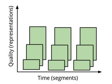
To prepare a video for adaptive video streaming with DASH, the video file is first encoded into different versions, each having a different rate and/or resolution. These are called representations or media presentations. The representations of a video all have the same content, but they differ in quality.

Each of these is further subdivided in time into segments of equal lengths (e.g., four seconds).

The content server then stores all of the segments of all of the representations (as separate files). Alongside these files, the content server stores a manifest file, called the Media Presentation Description (MPD). This is an XML file that identifies the various representations, identifies the video resolution and playback rate for each, and gives the location of every segment in each representation.

With these preparations complete, a user can begin to stream adaptive video from the server!

Once the MPD and video files are in place, users can start requesting DASH video.

First, the user requests the MPD file. It parses the MPD file, learns what representations are available, and decides what representation to request for the first segment. It then retrieves that specific file using the URL given in the MPD.

The user's device keeps a video buffer (at the application layer). As new segments are retrieved, they are placed in the buffer. As video is played back, it is removed from the buffer.

Each time a client finishes retrieving a file into the buffer, it makes a new decision as to what representation to get for the next segment.

For example, the client might request the following representations for the first four segments of video:

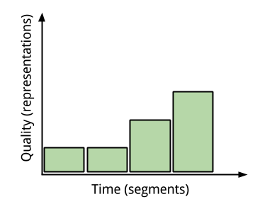
The cumulative set of decisions made by the client is called a decision policy. The decision policy is a set of rules that determine which representation to request, based on some kind of client state - for example, what the current download rate is, or how much video is currently stored in the buffer.

The decision policy is not specified in the DASH standard. Many decision policies have been proposed by researchers, each promising to deliver better quality than the next!

DASH decision policies

The obvious policy to maximize video quality alone would be to always retrive segments at the highest quality level. However, with this policy the user is likely to experience rebuffering - when playback is interrupted and the user has to wait for more video to be downloaded. This occurs when the video is being played back (and therefore, removed from the buffer) faster than it is being retrieved - i.e., the playback rate is higher than the download rate - so the buffer becomes empty. This state, which is known as buffer starvation, is obviously something we wish very much to avoid.

To create a positive user experience for streaming video, therefore, requires a delicate balancing act.

• On the one hand, increasing the video playback rate too much (so that it is higher than the download rate) causes the undesired rebuffers.
• On the other hand, decreasing the video playback rate also decreases the user-perceived video quality.

Performing rate selection to balance rebuffer avoidance and quality optimization is an ongoing tradeoff. Different DASH policies may make different decisions about how to balance that tradeoff. Different DASH policies may also decide to use different pieces of information for decision making. For example:

• A decision policy may decide to focus on download rate in its decision making - select the quality level for the next video segment according to the download rate from the previous segment(s).
• Or, a decision policy may focus on buffer occupancy (how much video is already downloaded into the buffer, waiting to be played back?) If there is already a lot of video in the buffer, the decision policy can afford to be aggressive in its quality selection, since it has a cushion to protect it from rebuffering. On the other hand, if there is not much video in the buffer, the decision policy should be careful not to select a quality level that is too optimistic, since it is at high risk of rebuffering.

Specific policies in this implementation

In this experiment, we will use an updated version of the DASH implementation developed for the following paper:

P. Juluri, V. Tamarapalli and D. Medhi, "SARA: Segment aware rate adaptation algorithm for dynamic adaptive streaming over HTTP," 2015 IEEE International Conference on Communication Workshop (ICCW), 2015, pp. 1765-1770, doi: 10.1109/ICCW.2015.7247436.

which you can browse on Github. It includes three DASH decision policies:

The "basic" policy is a rate-based policy that tries to keep the video rate at or below the current network data rate. You can see the "basic" implementation here.

The buffer-based rate adaptation ("netflix") algorithm uses the estimated network data rate only during the initial startup phase. Otherwise, it makes quality decisions based on the buffer occupancy, i.e. tring to avoid an empty buffer which would cause the video to freeze. It is based on the algorithm described in the following paper:

Te-Yuan Huang, Ramesh Johari, and Nick McKeown. 2013. Downton abbey without the hiccups: buffer-based rate adaptation for HTTP video streaming. In Proceedings of the 2013 ACM SIGCOMM workshop on Future human-centric multimedia networking (FhMN '13). Association for Computing Machinery, New York, NY, USA, 9–14. https://doi.org/10.1145/2491172.2491179

You can see the "Netflix" implementation here.

Finally, the segment-aware rate adaptation ("SARA") algorithm uses the actual size of the segment and data rate of the network to estimate the time it would take to download the next segment. Then, given the current buffer occupancy, it selects the best possible video quality while avoiding buffer starvation. It is described in

P. Juluri, V. Tamarapalli and D. Medhi, "SARA: Segment aware rate adaptation algorithm for dynamic adaptive streaming over HTTP," 2015 IEEE International Conference on Communication Workshop (ICCW), 2015, pp. 1765-1770, doi: 10.1109/ICCW.2015.7247436.

You can see the "SARA" implementation here.

Run my experiment

For this experiment, we will use three nodes, connected in a linear topology: a client, a router, and a server.

Follow the instructions for the testbed you are using (Cloudlab or FABRIC) to reserve the resources and log in to each of the hosts in this experiment.

git clone --recurse-submodules https://github.com/teaching-on-testbeds/adaptive-video.git 
cd adaptive-video  

Prepare the server

First, we will set up the “juliet” host as an adaptive video server. Open an SSH session on “juliet”, and run the commands in this section there.

At the server, we will set up an HTTP server which will serve the video files to the client.

First, install the Apache HTTP server:

sudo apt update
sudo apt install -y apache2

Then, download the video segments and put them in the web server directory:

wget https://nyu.box.com/shared/static/d6btpwf5lqmkqh53b52ynhmfthh2qtby.tgz -O media.tgz sudo tar -v -xzf media.tgz -C /var/www/html/

The web server directory now contains 4-second segments of the "open" video clip Big Buck Bunny, encoded at different quality levels. The Big Buck Bunny DASH dataset is from:

Stefan Lederer, Christopher Müller, and Christian Timmerer. 2012. Dynamic adaptive streaming over HTTP dataset. In Proceedings of the 3rd Multimedia Systems Conference (MMSys '12). Association for Computing Machinery, New York, NY, USA, 89–94. DOI:https://doi.org/10.1145/2155555.2155570

Prepare the router

Next, we will set up the router. Open an SSH session on “router”, and run the commands in this section there.

At the router, we will emulate different network conditions, to see how each DASH policy performs.

We will experiment with both a constant data rate, and a variable data rate like that experienced by a mobile user. For the mobile user, we'll use some network traces collected in the New York City metro area. With these traces, the data rate experienced by the DASH client in our experiment will mimic the experience of traveling around NYC on bus, subway, and ferry.

The NYC traces are shared from the following paper:

Lifan Mei, Runchen Hu, Houwei Cao, Yong Liu, Zifa Han, Feng Li & Jin Li. (2019, March). Realtime Mobile Bandwidth Prediction using LSTM Neural Networks. In International Conference on Passive and Active Network Measurement. Springer.

To download the traces, on the "router" node run:

git clone https://github.com/NYU-METS/Main nyc-traces

To extract the trace files from their compressed archive, we will need to install an appropriate utility:

sudo apt update
sudo apt install -y unrar-free

Then, run

unrar nyc-traces/Dataset/Dataset_1.rar

We will also download a couple of utility scripts to help us set a constant data rate or vary the data rate on the network. On the "router" node, run

wget https://raw.githubusercontent.com/teaching-on-testbeds/adaptive-video/main/rate-vary.sh -O ~/rate-vary.sh

and

wget https://raw.githubusercontent.com/teaching-on-testbeds/adaptive-video/main/rate-set.sh -O ~/rate-set.sh

Prepare the client

Finally, we need to prepare the “romeo” host as a video client. Open an SSH session on “romeo”, and run the commands in this section there.

Finally, we need to prepare the DASH client.

Download the AStream DASH video client on the "client" node:

git clone https://github.com/teaching-on-testbeds/AStream

We must install Python3 to run the DASH video client, and we will also install the video encoding utility ffmpeg so that we can reconstruct the video later:

sudo apt update
sudo apt install -y python3 ffmpeg

Now we are ready to run our experiments! We will run four experiments: one with a constant bit rate, one with a constant bit rate and an interruption in middle, one where we compare adaptive video policies under similar network conditions, and one with a varying bit rate using the NYC traces.

Experiment: constant bit rate

On the router, set a constant bit rate of 1000 Kbits/second with

bash rate-set.sh 1000Kbit

(The first time you run it, you may see an error referencing a problem deleting a qdisc, but you can safely ignore this error.)

Note: you can specify a data rate in Kbits/second using Kbit or in Mbits/second using Mbit.

Then, on the client ("romeo"), start the DASH player with the "basic" adaptation policy:

python3 ~/AStream/dist/client/dash_client.py -m http://juliet/media/BigBuckBunny/4sec/BigBuckBunny_4s.mpd -p 'basic' -d

(Note: you can alternatively try netflix or sara as the DASH policy.)

Leave this running for a while. Then, you can interrupt the DASH client with Ctrl+C.

To understand the performance of the DASH policy, we can look at the logs produced by the client. These will be located inside a directory named ASTREAM_LOGS in your home directory on the "client" node. Use

ls ~/ASTREAM_LOGS

to find these.

Use scp to retrieve the log with the .csv extension.

To help with data visualization, you can use this Python notebook. Follow the instructions to upload your log file, change the filename variable, and plot your results.

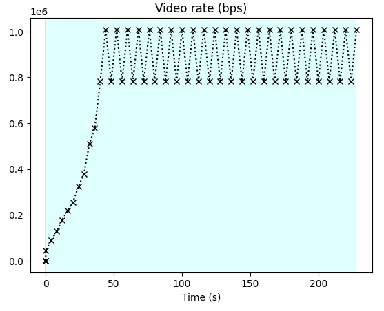
Here's an example. Note that initially, the video rate is low, but it increases after each segment as the network download rate continues to exceed the video rate. Eventually, it stabilizes around 1Mbps (the network download rate).

You can also re-create the video from the individual segments that were downloaded by the DASH client. The video segments will have been downloaded into a directory with the prefix TEMP in the "client" node's home directory. Find it with

ls ~

and then use cd to enter the directory.

To re-create the video, run

cat BigBuckBunny_4s_init.mp4 $(ls -vx BigBuckBunny_*.m4s) > BigBuckBunny_tmp.mp4 ffmpeg -i  BigBuckBunny_tmp.mp4 -c copy BigBuckBunny.mp4

Then, you can use scp to retrieve the BigBuckBunny.mp4 file from this directory, and play it back on your own computer.

Experiment: constant bit rate with interruption

In the experiment with constant bit rate, you may not have experienced any rebuffering.

To see how the video client works when there is a temporary interruption in the network, try repeating this experiment, but during the video session, reduce the network data rate to a very low value in middle of the session.

On the "router", set a constant bit rate of 1000 Kbits/second with

bash rate-set.sh 1000Kbit

Then, on the client ("romeo"), start the DASH player with the "basic" adaptation policy:

python3 ~/AStream/dist/client/dash_client.py -m http://juliet/media/BigBuckBunny/4sec/BigBuckBunny_4s.mpd -p 'basic' -d

Leave this running for one minute (60 seconds). Then, on the "router", reduce the network data rate to 100 Kbits/second:

bash rate-set.sh 100Kbit

After another 60 seconds, restore the original data rate:

bash rate-set.sh 1000Kbit

After a little while longer, stop the video client on "romeo" with Ctrl+C.

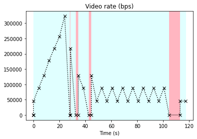
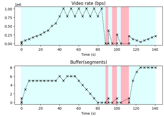
Repeat the data analysis. This time, you will note that when the network rate decreases, the buffer occupancy starts to drop, until it reaches zero and the client has to pause for rebuffering. When it is able to retrieve another segment, it will play it back, but if it has overestimated the download rate, then it will have to pause for rebuffering again. Eventually, the network data rate increases again, and then the video resumes playback at a higher rate and without interruptions.

Experiment: compare adaptive video policies

As in the previous experiment, in this experiment we will use a constant bit rate, with a brief interruption. However, we will compare the way two video adaptation policies react to this interruption - we'll compare a rate based policy (basic) and a buffer based policy (netflix) under identical settings (similar "high" network rate, "low" data rate, similar duration of the "high" data rate before the interruption, and and similar duration of the "interruption").

Rate-based vs. buffer-based policies

The basic rate adaptation policy (basic) chooses a video rate based on the observed download rate. It keeps track of the average download time for recent segments, and calculates a running average.

If the download rate exceeds the current video rate by some threshold, it may increase the video rate. If the download rate is lower than the current video rate, it decreases the video rate to ensure smooth playback.

You can see the source code for the basic policy here: basic_dash2.py

The buffer-based policy (netflix) adapts the video rate based on the current buffer occupancy, rather than the current download rate. When there are many segments already buffered, it can increase the video rate; if the buffer occupancy is low and the client is at risk of rebuffering, it must decrease the video rate.

You can see the source code for the netflix policy here: netflix_dash.py. This policy is based on the paper:

Te-Yuan Huang, Ramesh Johari, and Nick McKeown. 2013. Downton abbey without the hiccups: buffer-based rate adaptation for HTTP video streaming. In Proceedings of the 2013 ACM SIGCOMM workshop on Future human-centric multimedia networking (FhMN '13). Association for Computing Machinery, New York, NY, USA, 9–14. https://doi.org/10.1145/2491172.2491179

The policy defines two buffer occupancy thresholds: reservoir (defaults to 10%) and cushion (defaults to 90%). If the buffer occupancy is below the reservoir threshold, it selects the minimum video rate to fill the buffer quickly. If the buffer is within the reservoir and cushion range, it selects a video rate using a rate map function that maps buffer occupancy to video rate according to some increasing function. If the buffer occupancy exceeds the cushion threshold, it selects the maximum video rate.

The behavior of each policy is parameterized by the settings defined in the code base at: config_dash.py.

Key factors defined here for the rate based ("basic") policy include:

• BASIC_THRESHOLD - the maximum number of segments to store in the buffer in the rate based ("basic") policy.
• BASIC_UPPER_THRESHOLD - to avoid oscillations, in the rate based ("basic") policy, the video rate increases or decreases only if it is different from the download rate by at least this factor.
• BASIC_DELTA_COUNT - the number of segments' download rate to include in the moving average of network download rate. The smaller this number, the more reactive the client is to (potentially transient!) changes in network rate.

Key factors defined here for the buffer based ("netflix") policy include:

• NETFLIX_RESERVOIR - the value of the "reservoir" described above, as a fraction of total buffer size.
• NETFLIX_CUSHION - the value of the "cushion" described above, as a fraction of total buffer size.
• NETFLIX_BUFFER_SIZE - the maximum number of segments to store in the buffer in the buffer based ("netflix") policy.
• NETFLIX_INITIAL_BUFFER and NETFLIX_INITIAL_FACTOR - these define the behavior of the policy in the initial stage, which is a bit different than the approach described above.

Execute the experiment for the rate based policy

On the "router", we will configure the following "sequence" of network rates -

• 1000 Kbits/second for 100 seconds
• 350 Kbits/second for another 75 seconds
• 2000 Kbits/second for another 125 seconds

and while this is ongoing, we will run a DASH client with the rate based policy. After 300 seconds, we will stop the DASH client.

To realize this sequence of network rates, on the router, run

bash rate-set.sh 1000Kbit echo "Start the DASH client" sleep 100 bash rate-set.sh 350Kbit sleep 75 bash rate-set.sh 2000Kbit sleep 125 echo "Stop the DASH client"

On the client ("romeo"), immediately start the DASH player with the "basic" adaptation policy:

python3 ~/AStream/dist/client/dash_client.py -m http://juliet/media/BigBuckBunny/4sec/BigBuckBunny_4s.mpd -p 'basic' -d

Let the DASH player run for 300 seconds, then stop the video client on "romeo" with Ctrl+C.

Repeat the data analysis steps as before. Save the figures and the reconstructed video for the rate based policy, so that after completing the experiment in the next section with the buffer based policy, you can compare their behavior.

Execute the experiment for the buffer based policy

We will now repeat the same experiment for the buffer based policy.

On the router, run

bash rate-set.sh 1000Kbit echo "Start the DASH client" sleep 100 bash rate-set.sh 350Kbit sleep 75 bash rate-set.sh 2000Kbit sleep 125 echo "Stop the DASH client"

Then, on the client ("romeo"), start the DASH player with the "netflix" adaptation policy:

python3 ~/AStream/dist/client/dash_client.py -m http://juliet/media/BigBuckBunny/4sec/BigBuckBunny_4s.mpd -p 'netflix' -d

Let the DASH player run for 300 seconds, then stop the video client on "romeo" with Ctrl+C.

Repeat the data analysis steps as before. Save the figures and the reconstructed video for the buffer based policy, for comparison with the rate based policy in the previous section.

Experiment: mobile user

Finally, you can try to experience adaptive video as a mobile user! Repeat the experiment, but instead of setting a constant data rate on the router, you can let it play back a "trace" file with e.g.

bash rate-vary.sh ~/Dataset_1/Dataset/Ferry/Ferry5.csv 0.1

where the first argument is the path to a trace file, and the second argument is a scaling factor greater than 0 but less than 1. (The smaller the scaling factor, the lower the network quality while still preserving the trace dynamics.)

Then, on the client, run

python3 ~/AStream/dist/client/dash_client.py -m http://juliet/media/BigBuckBunny/4sec/BigBuckBunny_4s.mpd -p 'basic' -d

wait a minute or two, then stop the video player with Ctrl+C. Repeat the data analysis.

The following figure shows the "dynamics" (throughput in Mbps against time) for each of the traces:

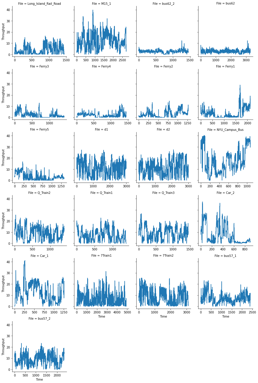
For some traces, the throughput is always more than enough to stream the video at the highest quality level. For the traces where the throughput is not sufficient to stream continuously at the highest quality level, a good decision policy should still be able to smooth over the variation in network quality and deliver high quality video without rebuffering.

Notes

Additional contributors and their contributions:

• Mayuri Upadhyaya - port GENI experiment to CloudLab, FABRIC, add exercises and suggestions on how to go further.
• Srishti Jaiswal (Summer of Reproducibility Fellow 2023) - update the AStream client for Python3 compatibility, and add the section on comparing adaptive video policies.